Motivation

Simulation helps us out when we want to find out more about real-world problems - like a crystal ball helping a wizard predict the future.

At YourMechanic, we face real world questions every day, such as:

• Should we hire more mechanics in X city?
• Should we add another hour of availability in Y city?
• Should we decrease padding time for mechanics?

What decisions should we make? Should we trust our intuition or rely solely on data? However, it takes time to accumulate enough data for us to evaluate the consequences. Nothing is worse than a strategy, proved to be a failure, that leads to an irreversible bad result.

A good simulation that precisely describes the real world business can carry out “pseudo experiments,” showing us the consequence within a negligible amount of time (and without causing any damage to our business). Ideally, the simulation magnifies the problem we are “debugging” in the business and guides us to the right direction.

Problem description

When potential customers come to visit YourMechanic via the web or app and enter data to get a quote, there is always the possibility that they won’t book an appointment. We want to learn more about the likelihood that people will (or won’t) book an appointment. What factors influence their decision? And, once we know these factors, how can we optimize them for greater conversion rates?

Exponential decay model

We start from a simple mathematical model:

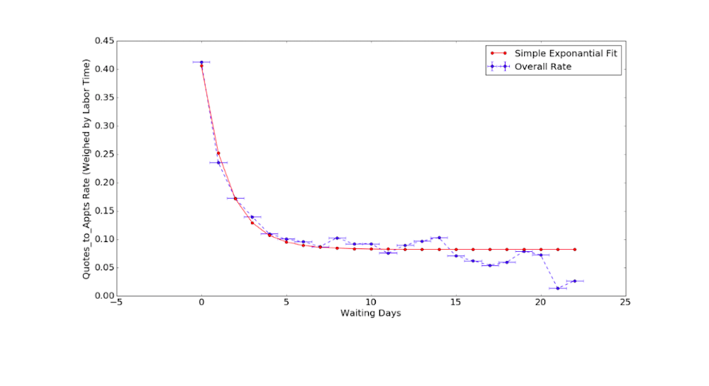
A visitor generates a quote, and we provide the available appointment dates and times. One key factor that determines the probability for the visitor to book is the wait time. This probability, P, can be described by the following equation:

As the wait time, t, gets longer, the probability decays exponentially. P_b is the base probability (the probability that a visitor is going to book an appointment no matter how long the wait time is). P₀+P_b is the maximum probability for the visitor to book, which should still be less than 1: some visitors come in just to get a price for comparison, and they have no real intention to book.

Figure 1. The probability of booking as a function of waiting times

We fit our simple model with real data, and feed it into the simulation.

God does play dice

Yes, in the simulated world, the programmer is the God who determines everything. We will roll a dice (generating a random number) three times for each quoting behavior. The first random number determines whether the simulated visitor would book an appointment or not. If he or she does, what time slot of which day should he or she choose?

Of course, the visitor can only book the available days. And I will roll the dice again to determine which available day will be chosen. As you can see in Figure 2, the customer (yes, he/she is a customer once he/she determines to book) tends to pick the earliest available day according to our data. And we fit this trend with a double-decay model:

Figure 2. The probability for a visitor to choose a certain available day

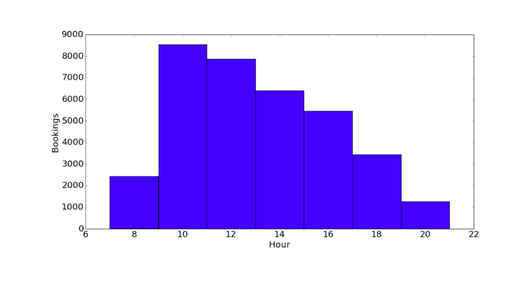
Then, we roll the dice for the third time to determine what time in the day the customer would prefer to have the service. This time, we feed in the real data, shown in Figure 3, and properly weighted it in the simulation.

Figure 3. The booking hour distribution for a certain period of data

Additional dimensions and unsupervised learning

Of course, real world is much more complicated than that -- the probability is related to the job type, the make, year, model, engine of the car, and other factors.

What’s more, someone might prefer the car to be serviced on a weekend while someone else may prefer evenings. Shall we provide more time slots available for them? More interesting and complex topics come into the play.

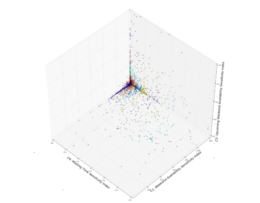
Figure 4: Each spot here corresponds to a make of car, and they are clustered into different groups (represented in different colors)

This is where we apply the machine-learning techniques. As an illustration, let’s look at Figure 4. To quantify the sensitivity to certain quantities, we introduce:

C0: index of waiting time sensitivity. This value is negative (as longer waiting days, the less probability a visitor is going to book). The lower this value is, the more sensitive the visitor is to the number of wait times.

C1: index of available weekend hours. The higher this value, the more likely this visitor is to book on available weekend hours.

C2: index of available hours in the upcoming weekend. The higher this value, the more likely that the visitor want to book the appointment in the upcoming weekend.

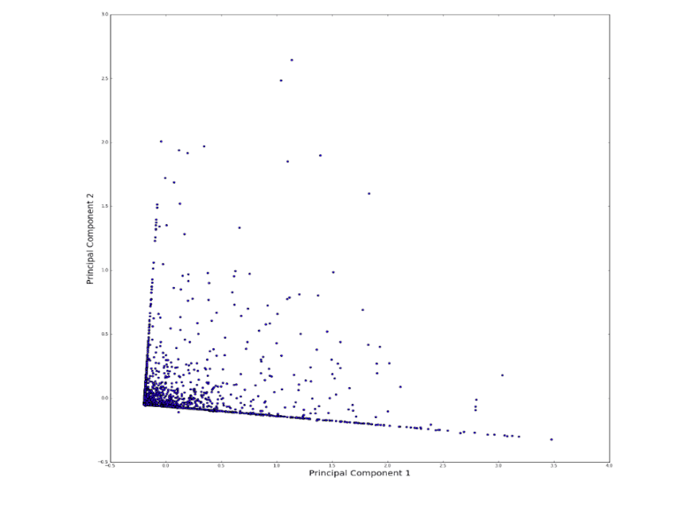
Use these three indices, we have defined a three-dimensional space (though the basis is not necessarily orthogonal to each other) yet. However, this is easy to deal with as long as we do a principal component analysis (PCA), as illustrated in Figure 5.

Figure 5. Two principal components of the three dimensions shown in Figure 4

Owners of different cars have different patience in waiting, these can be quantified in different parameters as we previously showed, and fed into simulation.

Running simulation

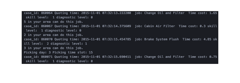
Now, let’s turn on the verbose printing in the simulation, and we see the following print out in the terminal:

Figure 6. The simulation is done on a quote basis. The probability of booking is calculated based on various features, and a random number is generated to determine this quote would become a booking. And the simulation determines the time slot of the appointment made by the “customer.”

Final words

With the help of the simulation framework, we are testing new algorithms in optimizing the mechanic schedule, and the first version tested with this simulation has been deployed. There are many other fascinating topics in data science; this simple simulation model example just scratches the surface. If this kind of analysis intrigues you, we are looking for smart and quantitative talents to join us and bring new ideas.